PID Controller

In this section, let us explore and understand this 17th century idea on how we could effectively do a speed control for the DC Motor, the PID Controller mechanism

PID Control

We will try to debunk a PID controller from a functional perspective and later on converge on the P, I and the D. The block diagram below shows the relation between a PID controller, and a process that is optimized by using a PID controller. The process here could be anything, but here we assume that the process here is a water heater control system (WHCS). The WHCS works by receiving a desired value for the temperature and heats the water. For example., if we want the WHCS to heat the water to 40° C, we want it to exactly do that.

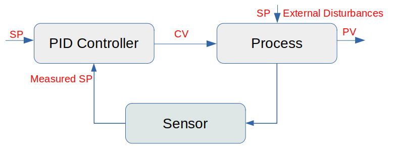
From the image above, we have the Process which emits a Process Value (PV), the PID Controller to which we give a Setpoint value (SP), the sensors that measure the actual Process Value (PV) which is then fed back into the PID controller, thus forming a closed loop. It can also be seen that the Process is also affected by external disturbances which makes it deviate from the Setpoint (SP). The PID controller's job is to account for these external disturbances and make the Process Value (PV) match the Setpoint (SP). For our case here where we want to do DC Motor speed control, we have something called a closed-loop controller, where we tell the controller how fast we want the motor to run. We call this the set point. The controller then measures the actual speed of the motor and calculates the difference between the actual speed, and the set point which is called the error. The controller then adjusts the voltage to the motor to reduce the error which in turn makes the Motor run at the set point we gave it originally.

If the SP and the PV are the same – then there is no other thing in this world that is going to be much happy than our PID controller. It does not have to do anything, it will set its output (the CV value from the image above) to zero, but in reality this is never going to be the case. So let us discuss further to understand the basics behind the PID controller.

We first need to understand what each of the term in the PID controller represent. The image below throws a bit of clarity on how each of the terms (Proportional, Integral & the Derivative) combine to get a smooth target output.

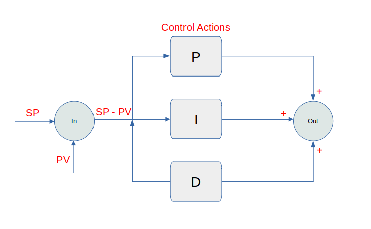
As we can see from the image above that the error is calculated by simply calculating the difference between the Setpoint (SV), and the Process Value (PV) or in other words, the error is simply the difference between the desired value and the actual value.

Let us now try to mathematically understand what each of the terms mean and how they influence in minimizing the error.

Proportional Control

This is the simplest of the control where the controller gives an output that is directly proportional to the current error (difference between SV and PV) times a proportional factor which is synonymous to the error value.

It can be seen from the equation above that with a small Kp the controller will make small attempts to minimize the error, while for a larger Kp, the controller will make a larger attempt to minimize the error. This is good, but this approach suffers from either an overshoot (if Kp is too large) or an undershoot (if Kp is too small). Both these effects, called the offset or the steady state error - we do want to avoid. There is always a steady state residual error in the case of a proportional controller. If this is too theoretical, let us understand it from a more practical perspective.

Imagive we have a water tank as shown in the image below with which our goal is to maintain a constant water level as defined by a Setpoint (SP) value. As long as the system is untouched, nothing changes but change is inevitable which means that the outflow will need to be increased, or the inflow need to be decreased or vice versa. But the goal remains constant which is to maintain the water levek in the tank at the given Setpoint value.

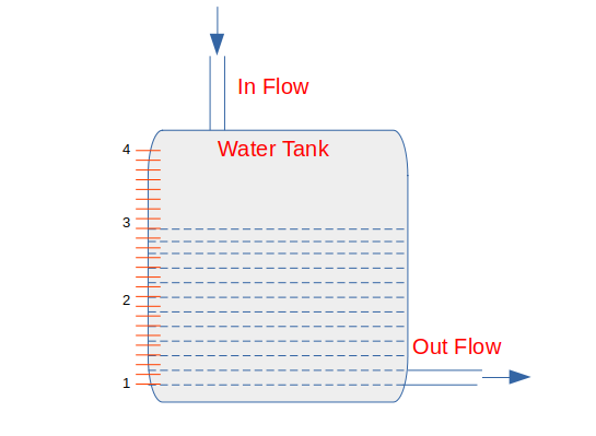
So with the goal of maintaining the Setpoint say at level 3, if we now increase the flow out of the tank, the tank level will start to decrease because of the imbalance between the inflow and outflow. While the tank level decreases, the error increases and the proportional controller will increase the controller output proportionally to this error. Consequently, the valve controlling the flow into the tank opens wider and more water flows into the tank.

As the water level continues to decrease, the error increases and valve continues to open until it gets to a point where the inflow again matches the outflow. At this point the tank level (and error) will remain constant. Because the error remains constant our proportinal controller will keep its output constant and the control valve will hold its position. The system now remains in balance, but the tank level remains below its set point. This remaining sustained error is called offset or the steady state error.

To get rid of this offset, the operator has to manually change the bias (the Kp term) such that the controller's output removes the offset. How can this be done automatically, that is exactly our next topic, the Integral controller!

Integral Control

By introducing a time component to the proportional controller, we can mitigate the overshoot and undershoot problems, which we termed as the offset or the steady state error. The integral controller, is capable of handling errors that happen over a certain set time interval. With using an integral component, we can thus overcome the steady state residual error that occurs with the proportional controller.

If the error is large enough, the integral controller will increment / decrement the controller output at a faster rate, while on the other hand if the error is small, the changes will be slow. For any given error, the speed of the integral action is set by the controller's time setting where a larget time setting results in slow integral action and vice versa.

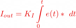
The equation above sums all the previous errors over a given time interval t and accounts for the error correction accordingly. If we have a larger value for the term Ki, it will result in an overshoot.

Differential Control or Derivative Control

The differential controller or the derivative (slope) controller is effectively used to predict the systems future behavior. It is mostly used for processes where motion control is needed, hence a good candidate for our Navo robot. The proportional and the integral controller both respond to past errors, the differential controller is capable of predicting future behavior of the error. As it can be seen from the equation below that the output of the differential controller depends on the rate of change of error over time, multiplied by a derivative constant Kd.

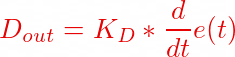
The output of the derivative this helps in reducing / minimizing the overshoot error. For example., a larger derivative or a larger slope indicates that the next error will be far away from the previous error but a small derivative or a smaller slope indicates that the next error will be likely close to the previous error.

PID Equation

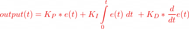
With the controllers and their equations nailed down, we have the following equations for the PID controller.

and by substituting the values, we get

So what that equation basically mean in our context which is to control the speed of the DC motor is that, the controller output is used to determine how much more or less the motor speed has to be adjusted so that the current speed (processValue) matches the target speed (setPoint). How does all this look like in reality? This is what we show in the code below:

 1unsigned long lastTime;
 2float processValue, output, setPoint;
 3float errorSum, previousError;
 4float kp, ki, kd;
 5int interval = 1000; //1 sec
 6
 7void pidControl()
 8{
 9   // Time interval to calculate the next error
10   unsigned long now = millis();
11   float timeDiff = (float)(now - lastTime);
12
13   if(timeDiff >= interval) 
14   {
15     // Calculate the error
16     float error = setPoint - processValue;
17     errorSum += error;
18     float dError = (error - previousError);
19  
20     // Calculate the PID control output
21     output = kp * error + ki * errorSum + kd * dError;
22  
23     // Memorize the variables for the next computation
24     previousError = error;
25     lastTime = now;
26   }
27}
28  
29void gainTuning(float Kp, float Ki, float Kd)
30{
31   kp = Kp;
32   ki = Ki;
33   kd = Kd;
34}

As it can be seen from the sketch above that we calculate the output of the controller using the pidControl() function which is called at regular intervals. That piece of code above does not deserve any further explanation, but a few points are worth mentioning and reasoning about.

Derivative kick

This happens when a change in the value of the error happens suddenly as a result of a change in the Setpoint. This in turn causes the derivative of the error to be instantaneously large enouch so that we see small spikes in our process output. This is not a big deal, but for systems where the change in Setpoint occurs more often, it is better that we address this to avoid putting stress in the system as such. A simple idea to overcome such derivative kick is to assume that the change in the Setpoint is constant, so the rate of change or in mathematical terms, the derivative of a constant (remember derivative is all about slope and for a constant there is no slope) is 0.

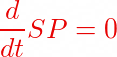
Using what we already know for the derivative control, let us use our assumption for a constant Setpoint to the derivative equation

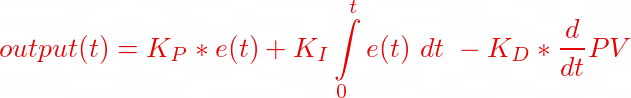
As it can be seen now that our derivative term becomes a measure of the Process value instead of the error term, hence our actual PID controller equation now becomes

It is easy to visualize this with some numbers and the resulting plat as shown in the image below.

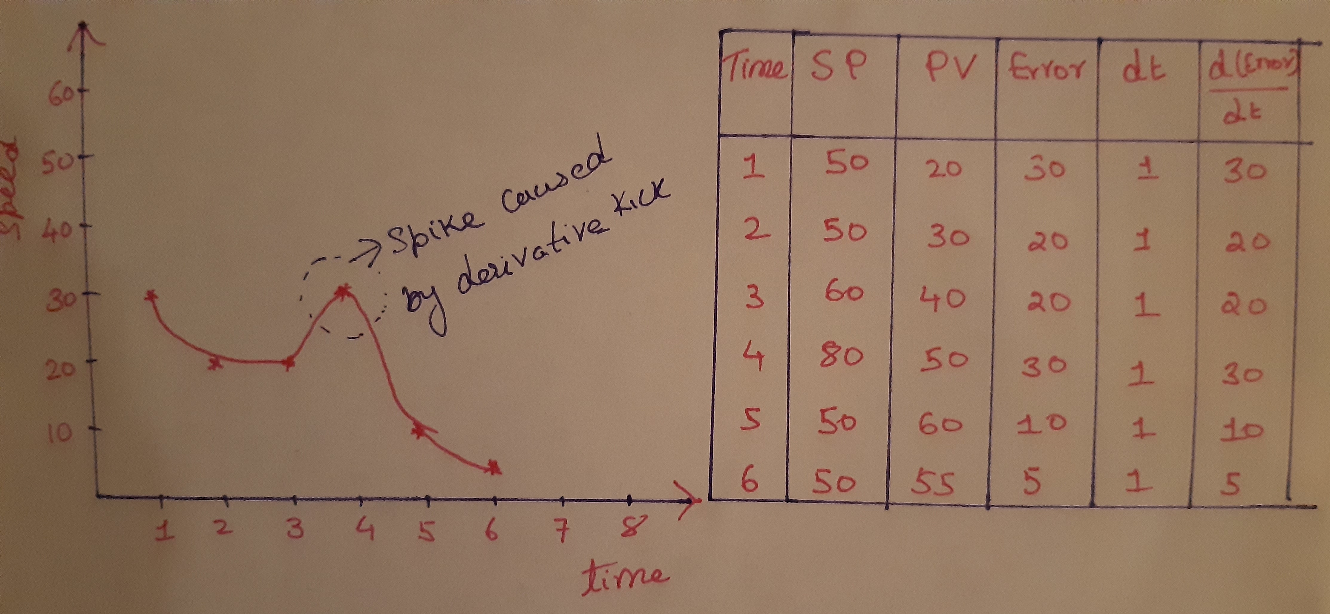
Looking at the plot between the derivative of the error vs time, It can be seen that as the Setpoint changes, it results in the error value to spike and this inturn causes the rate of change in error for a given time interval to result in a spike which we term the derivative kick. So by assuming that the Setpoint is a constant and derivating over the Process value actually helps to get rid of such a derivative kick.

PID Gain Tuning

Now one question might arise on what values to choose for the PID co-efficients. Luckily people have thought about this and the one that comes to mind is the Ziegler–Nichols method introduced by John G. Ziegler and Nathaniel B. Nichols in the 1940s. It is a heuristic technique of tuning a PID controller. The basic idea here is that it starts out by setting the integral and the derivative gains (basically the co-efficients Ki and Kd) to zero. The proportional gain (Kp) is then increased from zero until it reaches the ultimate gain Ku. This ultimate gain is the gain where the control loop has achieved a stable and consistent oscillation. The Ku and the oscillation period is then used to set the P, I and the D gains effectively. Let us not dive more into this for now.

Tuning the parameters or the gain in a running system is a topic in itself.

Hope I was able to explain the PID controller mechanism! With this basic understanding, head over here to see how we could combine all what we have learnt theoretically so far to a more practical example.